Physical and Chemical

1.4

Variability in ocean currents around Australia

Contributors

Charitha B. Pattiaratchi1,2

Prescilla Siji1,2

1 Oceans Graduate School, The University of Western Australia, Perth, WA, Australia
2 UWA Oceans Institute, The University of Western Australia, Perth, WA, Australia

Key Information

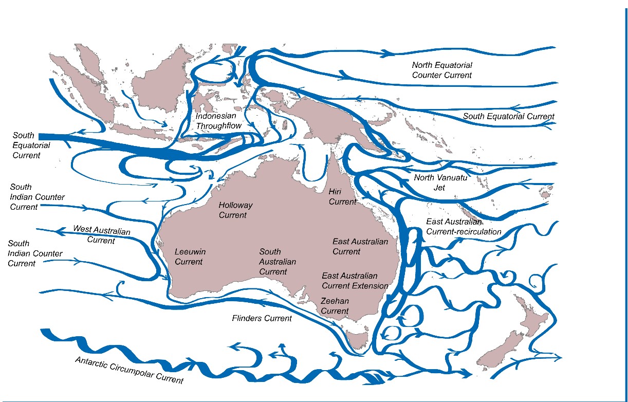
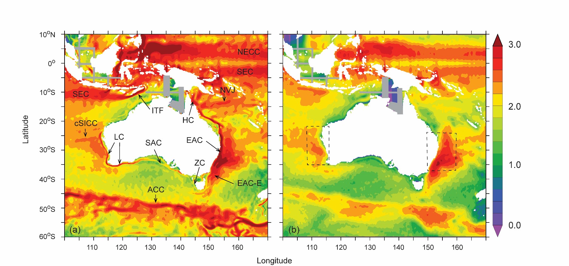
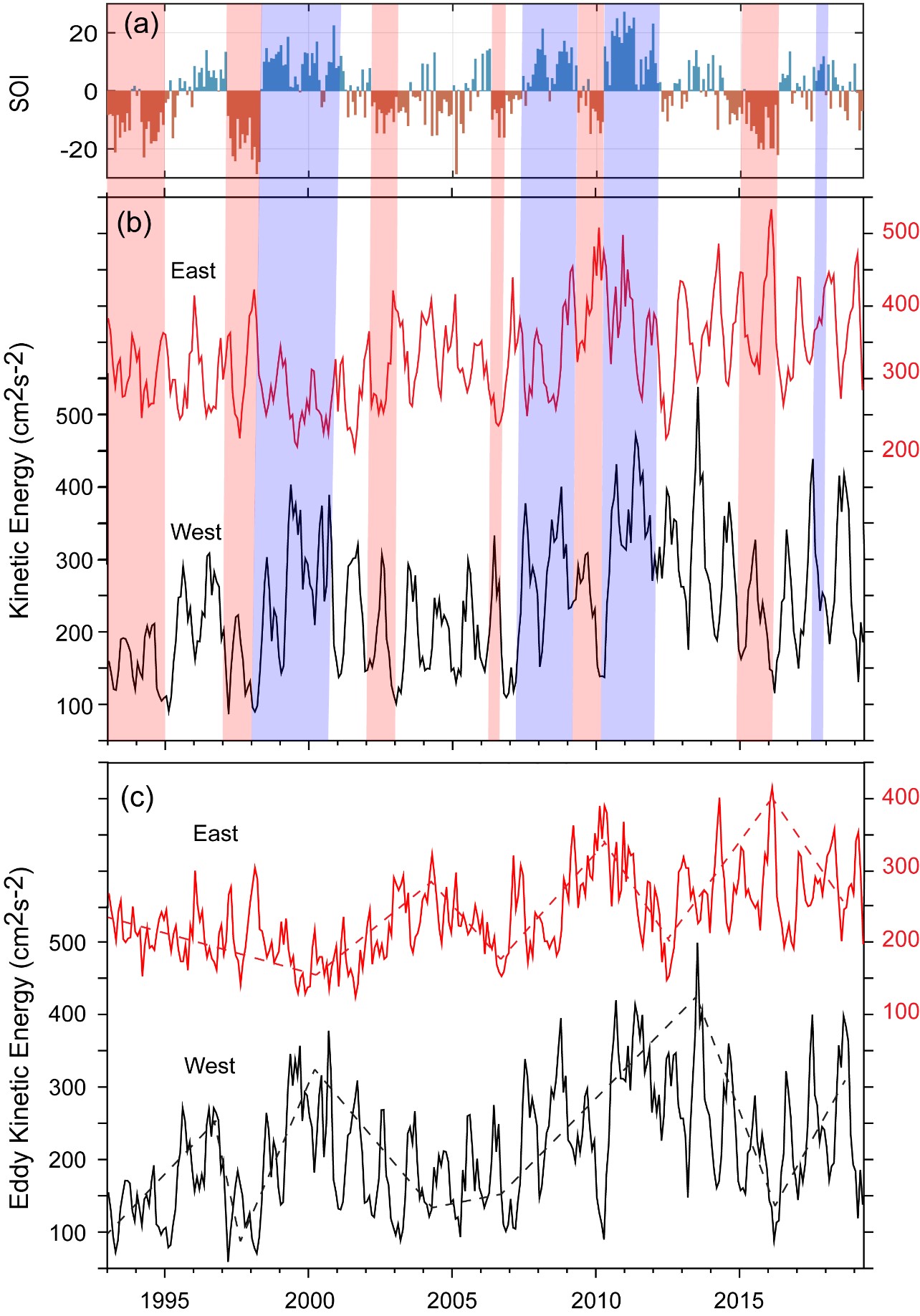
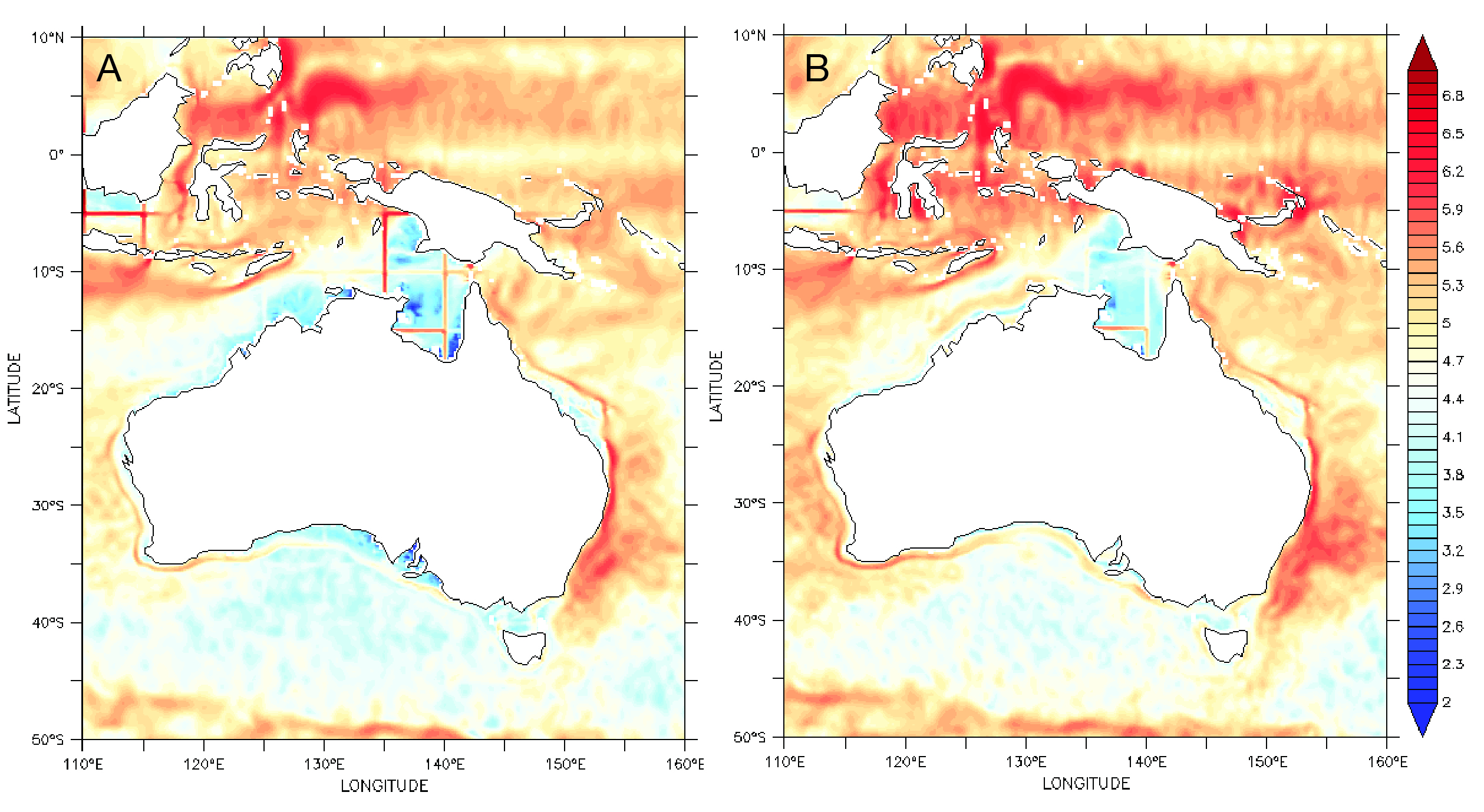
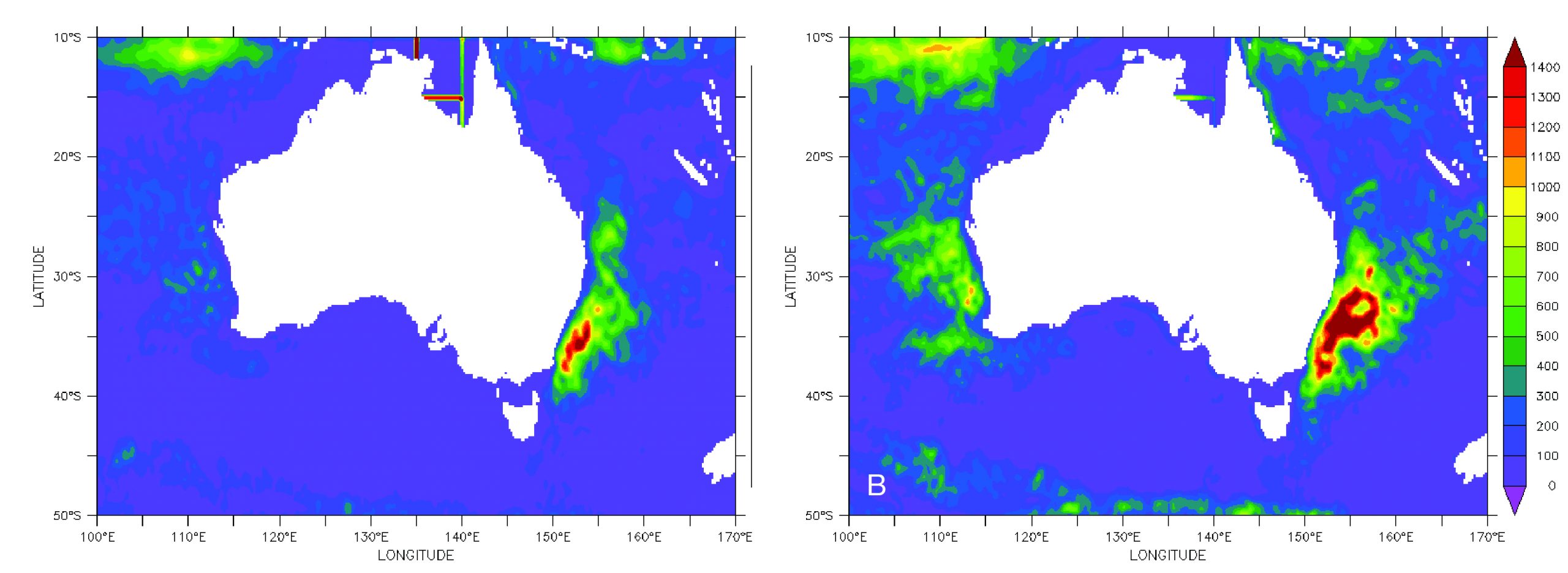
Ocean currents also have a strong influence on marine ecosystems, through the transport of heat, nutrients, phytoplankton, zooplankton and larvae of most marine animals. We used geostrophic currents derived satellite altimetry measurements between 1993 and 2019 to examine the Kinetic Energy (KE, measure of current intensity) and Eddy Kinetic Energy (EKE, variability of the currents relative to a mean) around Australia. The East Australian (EAC) and Leeuwin (LC) current systems along the east and west coasts demonstrated strong seasonal and inter-annual variability linked to El Niño and La Niña events.  The variability in the LC system was larger than for the EAC. All major boundary currents around Australia were enhanced during the 2011 La Niña event.

Keywords

La Niña, El Niño, East Australian Current, Leeuwin Current

Variability in ocean currents around Australia

Ocean currents play a key role in determining the distribution of heat across the planet, not only regulating and stabilising climate, but also contributing to climate variability. Ocean currents also have a strong influence on marine ecosystems, through the transport of phytoplankton (primary producers), zooplankton (grazers on the primary producers and food for higher trophic levels), and larvae of most marine animals. Ocean currents also regulate the physiology and growth of marine life by controlling ambient conditions through the redistribution of heat and nutrients.

The island continent of Australia is surrounded by surface and subsurface boundary currents that flow along the continental shelf and slope. The unique feature of this circulation is that along both east and west coasts, boundary currents transport warm-water southward via the East Australian (EAC) and Leeuwin Currents (LC), respectively  (Wijeratne, Pattiaratchi, & Proctor, 2018). These boundary currents are enhanced through inflows from the south Pacific and south Indian Ocean basins. Australia’s boundary currents are an important conduit for the poleward heat and mass transport and inter-ocean water exchange in the tropics (Indonesian Throughflow; Sprintall, Wijffels, Molcard, & Jaya, 2009) and the sub-tropics (Tasman outflow; Hu et al., 2015; van Sebille, England, Zika, & Sloyan, 2012). Major surface boundary currents include the Indonesian Throughflow, Holloway, Leeuwin, South Australian, Flinders, Zeehan, East Australian and Hiri currents (Figure 1).

Previous studies have highlighted the seasonal and inter-annual variability associated with the LC, with stronger (weaker) currents during the winter (summer) and La Niña (El Niño) events (Feng, Meyers, Pearce, & Wijffels, 2003; Pattiaratchi & Buchan, 1991; Wijeratne et al., 2018). The ENSO (El Niño Southern Oscillation) signal within the LC is transmitted along the south coast of Australia, where there is enhanced upwelling off Kangaroo Island (Middleton et al., 2007). EAC is stronger during summer and slightly weaker during winter (Wijeratne et al., 2018), with decadal ENSO variations affecting the EAC transport variability (Holbrook, Goodwin, McGregor, Molina, & Power, 2011). Variability associated with ENSO along east coast of Australia appears to be weaker than along the west coast.

Satellite altimeter observations provide a synoptic view of the ocean variability at different time and space scales. Sea surface height data provide information on geostrophic surface flow and thus Kinetic Energy (KE) and the intensity of the surface current variability activity through the Eddy Kinetic Energy (EKE, the variance of geostrophic surface velocities). KE is thus a measure of the intensity of currents, whilst EKE provides variability of the currents relative to a mean. Thus, changes in KE and EKE over time determine the inter-annual variability of the ocean currents. Many studies have examined the variability of EKE in the ocean using altimeter data (Caballero, Pascual, Dibarboure, & Espino, 2008; Ducet, Le Traon, & Reverdin, 2000; Ludicone, Santoler, Marullo, & Gerosa, 1998; Pujol & Larnicol, 2005).  

To calculate KE and EKE of ocean currents around Australia, we used global ocean reanalysis of altimeter data (AODN dataset: “IMOS - OceanCurrent - Gridded sea level anomaly - Delayed mode”). For the period January 1993 to December 2010, geostrophic current components were only available on alternative days. Data were interpolated to create a daily mean data set. For the period January 2011 to April 2019, daily mean data were available and no interpolation was necessary. Daily mean data for the period January 1993 to April 2019 were then used to create monthly mean data. The KE for each month was defined as (Caballero et al., 2008):

KE = 1/2 √u²+v²   

where, u and v were the monthly mean of zonal (east-west) and meridional (north-south) geostrophic current components respectively. The EKE was defined as:

EKE = 1/2 √u’²+v’²

where u = u - U and v = v' - V , with U and V are the monthly climatological means of the zonal and meridional velocity components, respectively.

Monthly KE and EKE were used to obtain the area average in two regions on the east (24°–37.5°S, 150°–160°E) and west coasts of Australia (21°–36°S, 108°–116°E, Figure 2).

Mean KE from 1993-2019 indicated that all major boundary currents around Australia and inflows were captured in the altimeter data. Boundary currents along the east coast (Hiri, EAC, EAC-extension, EAC-recirculation), as well as the main inflow (North Vanuatu Jet), were well defined (Figure 2a). Similarly, boundary currents along the west coast (Holloway, Leeuwin, South Australian and Zeehan Currents), as well as the main inflows (Indonesian Throughflow, central South Indian Counter Current) were also well defined. The EKE also indicated regions of high variability along the east and west coasts of Australia, equatorial regions and the Antarctic Circumpolar Current (Figure 2b).

The monthly mean time series of KE and EKE for the regions along the east and west coasts (Figure 2b) highlighted the strong seasonal variability (Figure 3b,c). The east and west time series were out-of-phase, reflecting that the EAC is strongest in January, whist the LC is strongest in June. It was also noticeable that the seasonal variability (i.e., the seasonal range in both KE and EKE) was higher along the west than the east coast, indicating greater seasonal variability in the LC than the EAC. For example, the maximum seasonal range for KE (EKE) was 370 (350) cm2s-2 for the west coast (in 2013), but only 270 (220) cm2s-2 for the east coast (in 2016). Differences in the seasonal variability between the east and west coasts was more pronounced for EKE than KE (Figure 3c).

Over the study period, the range of the KE for east and west coasts were different; for the east coast, the range was 340 cm2s-2 (200-540 cm2s-2), whilst for the west coast the range was 450 cm2s-2 (90-540 cm2s-2). Similarly, for EKE, ranges were 310 cm2s-2 (60-370 cm2s-2) and 440 cm2s-2 (60-500 cm2s-2), for east and west coasts, respectively (Figure 3). This indicates that the inter-annual variability in the LC syatem was larger than the EAC.

The variability in both KE and EKE demonstrated that the EAC and LC undergo strong inter-annual variability related to ENSO events (Figure 3b). The EAC appears to be stronger towards the waning phase of El Niño events (e.g., January in 1998, 2003, 2010, 2016). For EAC, highest (lowest) KE and EKE were during the 2016 and 2010 El Niño (1998 La Niña) events. By contrast, both KE and EKE increased (decreased) during La Niña (El Niño) events. These periods of strong (weak) KE and EKE corresponded to warm (cold) SST anomalies along both coasts (see State and Trends of Australia’s Ocean report 1.2: Sea surface temperature variability).

In addition to variability associated with ENSO events, there were also trends in both KE and EKE time series over a 7-10 year period. In the east, there were decreasing trends in 1993-2000, 2005-2007, 2010-2013 and 2016-2019 (Figure 3c). By contrast, there were increasing trends in 2001-2005, 2007-2010 and 2013-2016 (Figure 3c). Here, changes in the trend were associated with the occurrence of ENSO events with maxima (minima) during El Niño (La Niña) events.  Similar changes were observed in the west, with decreasing trends during 1996-1997, 2000-2004, 2013-2016 and increasing trends during 1993-1993, 1997-2000, 2004-2013 and 2016-2018. Changes in the trends were also associated with ENSO events, but in an opposite sense, with maxima (minima) during La Niña (El Niño) events (Figure 3c).  An interesting feature along the west coast was that from 2002-2008, both KE and EKE were relatively low over several years, indicating weaker LC during this period.

The influence of ENSO events around Australia is highlighted by examining the annual mean KE and EKE distributions for 2006 (weak El Niño) and 2011 (La Niña) events (Figure 4). A noteworthy feature is that all major boundary currents in the west were enhanced in 2011 compared to 2006. These include the Indonesian Throughflow, LC, and the offshore west coast. However, two regions have significant changes in KE. In the north, the KE associated with the Holloway Current increased during 2011 (cf. Figures 4a,b). In the south, KE associated with the LC and South Australian Current increased, with the whole Great Australian Bight having higher KE in 2011 and indicating a northward migration of the LC into the GAB. In the east, the EAC had similar KE values. This was due to the 2011 La Niña following the 2009-10 El Niño, with KE and EKE in the east remaining higher during 2011 (Figure 3). The main changes were in the Coral Sea, with higher values in 2011. Similarly, the EKE increased in 2011 compared to 2006 along both the east and west coasts, as well as in the Indonesian Throughflow and Antarctic Circumpolar Current (Figure 5a,b).

Ocean currents – with their key role in transporting water with different temperature/salinity characteristics, nutrients and biota – are critical for regional climate and marine ecosystem function. Variability in these current systems has significant influence on year-to-year changes in biomass of marine life. The analysis of KE, as a measure of the intensity of the currents, and EKE as a measure of the variability in the currents over time, provide useful insights into observed changes in marine systems. One of the best examples of the role of ocean currents is their influence on marine heatwaves that can have devastating effects on the marine environment, and their frequency and intensity appears to be increasing (Babcock et al., 2019). In 2011, an extreme heatwave off the coast of Western Australia had a devastating effect on the marine system, particularly seagrass, rock lobster and scallops. There was also a substantial decline in zooplankton biomass, abundance and size, and an increase in diversity (see State and Trends of Australia’s Ocean Report 4.2: The impact on zooplankton of the 2011 heatwave off Western Australia). This was during the 2011 La Niña event, defined as the Ningaloo Niña, where the unseasonal strengthening of the LC occurred earlier in the year (February), transporting warmer water southward. Southerly winds that bring colder water to the surface through upwelling also decreased during this period. The continuing stronger LC through to 2013 maintained the warm water, which continued to impact corals (Babcock et al., 2019).  Similarly, warm SST anomalies along the east coast were also associated with the 1997-98 El Niño events and importantly the extended period of warming from 2014 to 2018 were associated with a stronger EAC.

The western rock lobster (Panulirus Cygnus) is Australia's most valuable wild-caught commercial fishery. When released, rock lobster larvae (phyllosoma) spend up to 11 months in the deep ocean (offshore LC) before ocean currents transport them to the coast. The abundance of puerulus (late stage phyllosoma) is used as a reliable predictor of the lobster catch for the fishery 3-4 years in advance. For many years, there was a strong relationship between the mean Fremantle sea level, as a proxy for the strength of the Leeuwin Current, and the settlement of puerulus (Pearce & Phillips, 1988). However, since 2001, the relationship between mean sea level and rock lobster recruitment has diminished, with unprecedented low settlement numbers in 2008 (de Lestang et al., 2015). The time series indicate that prior to 2008, both KE and EKE were relatively low, suggesting that lower KE and EKE over several years could have a substantial influence on the cross-shelf transport that contribute to the transport of puerulus onshore.

Babcock, R. C., Bustamante, R. H., Fulton, E. A., Fulton, D. J., Haywood, M. D. E., Hobday, A. J., . . . Vanderklift, M. A. (2019). Severe continental-scale impacts of climate change are happening now: extreme climate events impact marine habitat forming communities along 45% of Australia’s coast. Frontiers in Marine Science, 6(411). doi:10.3389/fmars.2019.00411

Caballero, A., Pascual, A., Dibarboure, G., & Espino, M. (2008). Sea level and Eddy Kinetic Energy variability in the Bay of Biscay, inferred from satellite altimeter data. Journal of Marine Systems, 72(1-4), 116-134. doi:10.1016/j.jmarsys.2007.03.011

Ducet, N., Le Traon, P. Y., & Reverdin, G. (2000). Global high-resolution mapping of ocean circulation from TOPEX/Poseidon and ERS-1 and-2. Journal of Geophysical Research-Oceans, 105(C8), 19477-19498. doi:10.1029/2000jc900063

De Lestang, S., Caputi, N., Feng, M., Denham, A., Penn, J., Slawinski, D., Pearce, A., How J. (2015). What caused seven consecutive years of low puerulus settlement in the western rock lobster fishery of Western Australia? ICES Journal of Marine Science, 72, 59-59.

Feng, M., Meyers, G., Pearce, A., & Wijffels, S. (2003). Annual and interannual variations of the Leeuwin Current at 32°S. Journal of Geophysical Research, 108(C11), 3355. doi:doi:10.1029/2002JC001763

Holbrook, N. J., Goodwin, I. D., McGregor, S., Molina, E., & Power, S. B. (2011). ENSO to multi-decadal time scale changes in East Australian Current transports and Fort Denison sea level: Oceanic Rossby waves as the connecting mechanism. Deep-Sea Research Part Ii-Topical Studies in Oceanography, 58(5), 547-558. doi:10.1016/j.dsr2.2010.06.007

Hu, D. X., Wu, L. X., Cai, W. J., Sen Gupta, A., Ganachaud, A., Qiu, B., . . . Kessler, W. S. (2015). Pacific western boundary currents and their roles in climate. Nature, 522(7556), 299-308. doi:10.1038/nature14504

Ludicone, D., Santoler, R., Marullo, S., & Gerosa, P. (1998). Sea level variability and surface eddy statistics in the Mediterranean Sea from TOPEX/POSEIDON data. Journal of Geophysical Research, 103(C2), 2995-3011.

Middleton, J. F., Arthur, C., Van Ruth, P., Ward, T. M., McClean, J. L., Maltrud, M. E., . . . Middleton, S. (2007). El Nino effects and upwelling off South Australia. Journal of Physical Oceanography, 37(10), 2458-2477. doi:10.1175/jpo3119.1

Pattiaratchi, C. B., & Buchan, S. J. (1991). Implications of long-term climate change for the Leeuwin current. Journal of the Royal Society of Western Australia, 74, 133-140.

Pearce, A. F., & Phillips, B. F. (1988). ENSO events, the Leeuwin current, and larval recruitment of the western rock lobster. Journal Du Conseil, 45(1), 13-21. Retrieved from <Go to ISI>://WOS:A1988Q548000002

Pujol, M. I., & Larnicol, G. (2005). Mediterranean sea eddy kinetic energy variability from 11 years of altimetric data. Journal of Marine Systems, 58(3-4), 121-142. doi:10.1016/j.jmarsys.2005.07.005

Sprintall, J., Wijffels, S. E., Molcard, R., & Jaya, I. (2009). Direct estimates of the Indonesian throughflow entering the Indian Ocean: 2004–2006. Journal of Geophysical Research (oceans), 114.

van Sebille, E., England, M. H., Zika, J. D., & Sloyan, B. M. (2012). Tasman leakage in a fine-resolution ocean model. Geophysical Research Letters, 39, 5. doi:10.1029/2012gl051004

Wijeratne, S., Pattiaratchi, C., & Proctor, R. (2018). Estimates of surface and subsurface boundary current transport around Australia. Journal of Geophysical Research-Oceans, 123(5), 3444-3466. doi:10.1029/2017jc013221

Figure 1

Mean surface currents around Australia (modified from (Wijeratne et al., 2018).

Figure 2

Mean (a) kinetic energy and, (b) eddy kinetic energy for the oceans around Australia over the period 1993-2018. The current systems in (a) are: ITF= Indonesian Throughflow; SEC=South Equatorial Current; HLC=Holloway Current; LC=Leeuwin Current; cSICC= central South Indian Counter Current; ACC=Antarctic Circumpolar Current; SAC=South Australian Current; EAC=East Australian Current; EAC-E=East Australian Current Extension; NVJ=North Vanuatu Jet; HC=Hiri Current; NECC=North Equatorial Counter Current; ZC = Zeehan Current. The location of the boxes where means were calculated are shown in (b) as dashed lines. Grey lines represent missing data.

Figure 3

Time series of (a) Southern Oscillation Index (SOI), (b) monthly mean kinetic energy, and (c) eddy kinetic energy from January 1993-April 2019. The red line is for the eastern box and the black line is for the western box. Note that the time series for the eastern box has been shifted by +300 cm2s2 to separate the two time series as shown the scale on right. Red and Blue shaded lines represent El Niño and La Niña events, respectively. Dashed lines (c) indicate the linear trend.

Figure 4

Annual mean kinetic energy for (a) 2006 (El Niño), and (b) 2011 (La Niña). Note the logarithmic scale is with units log(cm2s-2).

Figure 5

Annual mean eddy kinetic energy for (a) 2006 (El Niño), and (b) 2011 (La Niña). Note the linear scale with units cm2s-2).

Download this Time Series Report

Citing this report: 

Pattiaratchi C.B, Siji P. (2020) Variability in ocean currents around Australia. In Richardson A.J, Eriksen R, Moltmann T, Hodgson-Johnston I, Wallis J.R. (Eds). State and Trends of Australia’s Ocean Report. doi: 10.26198/5e16a2ae49e76

doi: 10.26198/5e16a2ae49e76

Access the Data

Access the data that contributes to this time-series by clicking the icons below

11. SRS-02

Satellite Remote Sensing

Citing the Report

Richardson A.J, Eriksen R, Moltmann T, Hodgson-Johnston I, Wallis J.R. (2020). State and Trends of Australia’s Ocean Report, Integrated Marine Observing System (IMOS).

IMOS_logo-stacked-reversed-01

The State and Trends of Australia's Ocean Report was supported by IMOS. IMOS gratefully acknowledges the additional support provided by the Commonwealth Scientific and Industrial Research Organisation (CSIRO).

The State and Trends of Australia's Ocean website is maintained by IMOS.


NCRIS-PROVIDER-REV

Australia’s Integrated Marine Observing System (IMOS) is enabled by the National Collaborative Research Infrastructure Strategy (NCRIS). It is operated by a consortium of institutions as an unincorporated joint venture, with the University of Tasmania as Lead Agent.

Disclaimer:

You accept all risks and responsibility for losses, damages, costs and other consequences resulting directly or indirectly from using this site and any information or material available from it. While the Integrated Marine Observing System (IMOS) has taken reasonable steps to ensure that the information on this website and related publication is correct, it provides no warranty or guarantee that information provided by the authors is accurate, complete or up-to-date. IMOS does not accept any responsibility or liability for any actions taken as a result of, or in reliance on, information on its website or publication. Users should check with the originating authors to confirm the accuracy of the information before taking any action in reliance on that information.

If you believe any information on this website or in the related publication is inaccurate, out of date or misleading, please bring it to our attention by contacting the authors directly or emailing us at IMOS@imos.org.au


Images and Information:

All information on this website remains the property of those who authored it. All images on this website are licensed through Adobe Stock, Shutterstock, or have permission from the original owner.